The GDelt database 1, on 18-11-2019, consists of 492,618 segments. Processing the top 10 most mentioned topics for each date on the whole data set would take a long time. Using clusters in the cloud, like AWS EMR, significantly decreases up the needed computation time but might be costly. To make the best use of the clusters on AWS EMR a minimization of the idle time of the machines is desired.
Before running the implementation on all segments of the GDelt database on a big cluster, we
were careful with the resources when scaling up. We started off by
making sure the implementation works on 1 master and 2 worker nodes of
type m4.large. After we had a succesful run on a handful of segments,
we scaled towards 1 master and 5 worker nodes of type c4.8xlarge on
12, 24, 48 and 96 segments. Apparently the overhead was significant,
since each of the jobs took around 50 seconds. Since all bugs were
fixed, we were confident to scale up some more. Results on 1000 and 10000 segments are shown below.
| Number of segments | (Expected) Run time |
|---|---|
| 1000 | 1 min 20 sec |
| 10000 | 2 min 26 sec |
| 157378 | 12 min 21 sec |
Using the runtimes of 1000 and 10000 segments we can estimate how long it would take to run the whole set.
A linear function y = (19/4500)x+(682/9) gives us the value for the whole dataset (12 min 21 sec).
Implementation
Custom function
Our initial DataFrame-implementation had a decent scaling behavior.
But when calling explain in an attempt to find a way to improve it, we
realized that a custom function to retrieve only the top 10 results of
each date could be a bottleneck. We substituted this custom function for
the SQL built-in rank function. See the code snippet below:
spark.sql("CREATE TEMPORARY VIEW View5 AS
	SELECT * FROM (
		SELECT date, newtopic, totalCount,
		rank() OVER (PARTITION BY date ORDER BY totalCount desc) AS rank
		FROM View4)
   WHERE rank <= 10)
Since rank() is a native SQL-function, the Catalyst Optimizer can take
it into account when optimizing the execution plan.
Distribute by date
In order to avoid two shuffles, we partition the data by date early in the process. Therefore, all data needed to output the top 10 names for a date is already on the same partition, so another shuffle is not needed. This is done by the code in the snippet below:
spark.sql("CREATE TEMPORARY VIEW View1 AS SELECT * FROM View0 DISTRIBUTE BY DATE")
It is hard to precisely capture the significance of the improvement, because it is hard to see exactly what is going on on each of the cores of the cluster. However, we do believe that this change has significant impact, especially when the amount of data is very large, since shuffles are usually becoming more expensive on larger amounts of data.
Tuning
There are multiple things that we tried to optimize the performance. We tried to use the Kryo serializer for lower I/O overhead. We also tried to partition the data in a smart way, such that it fits to the cluster configuration at hand.
Kryo
Scala Spark applications use the Java serializer by default. However,
using the Kryo serializer might make I/O operations and network traffic
more efficient. We did a small experiment on 480 segments with 1 master
and 5 worker nodes of type c4.8xlarge with the Kryo serializer and the
default Java serializer. The results are shown in the table below.
| Serializer | Comparison 1 | Comparison 2 | Comparison 3 |
|---|---|---|---|
| Kryo | 1m21s | 56s | 58s |
| Java | 1m07s | 52s | 53s |
Kryo vs Java serialization in queries on 480 segments with 1 master
and 5 worker nodes of type c4.8xlarge.
Switching to the Kryo serializer might not help in this case, because
the objects that are serialized consist of only two Strings (date and
name) and an Integer (count). The simplicity of the classes does not
unlock Kryo’s full potential. Another experiment confirms this: with 1
master and 20 worker nodes of c4.8xlarge on 5760 segments the
execution time is 102 and 90 seconds with the Kryo and Java serializer
respectively.
Partitioning
We have also investigated how we could optimize the number of
partitions. Using the spark history server, we have seen that the last
stage is divided into 200 partitions. Since we are using 20 machines
with 36 vCores each, we could process 20 * 36 = 720 partitions in parallel.
That means that 520 vCores are not used in the final stage. Therefore,
we tried scaling down the cluster size to 6 c4.8xlarge machines, with
6 * 36 = 216 vCores in total, just enough to process all partitions in the
last stage in parallel. The consequence is that the processes in earlier
stages also have access to only 216 vCores, so this will take longer,
but the overall idleness of the machines might be lower.
The level of parallelism to use in a spark cluster is advised2 to be
2 or 3 times the number of vCores. Using this heuristic we get the
number of partitions to be 216 vCores * 3 = 648 partitions for the other
tasks.
Comparison
To compare different setups, we have summarized them below. To calculate the price of the computation, we used the fixed price of the Amazon EC2 instances. The idle cost is the cost wasted to the idleness of the cluster.
| Cluster Configuration | Tuning | Runtime | Idleness | Costs | Idle cost |
|---|---|---|---|---|---|
| 20 worker c4.8xlarge, 1 master c4.8xlarge | No tuning | 4m24s | 51.41% | $0.3960 | $0.2036 |
| 20 worker c5.2xlarge, 1 master c4.8xlarge | Slower machines to increase utilization | 14m24s | 30.26% | $0.5184 | $0.1569 |
| 14 worker c5.2xlarge, 1 master m5.xlarge | Number of partitions set to 3*#vCPUs | 21m35s | 31.68% | $0.5439 | $0.1723 |
| 6 worker c4.8xlarge, 1 master m5.xlarge | Number of partitions set to 3*#vCPUs. Number of machines (6) as wide as the last job of the computation. | 16m43s | 43.08% | $0.4514 | $0.1945 |
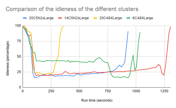
To compare the different cluster setups we also analyzed the average idleness and the average load ratio (number of procs divided by number of vCPU’s) of the clusters.
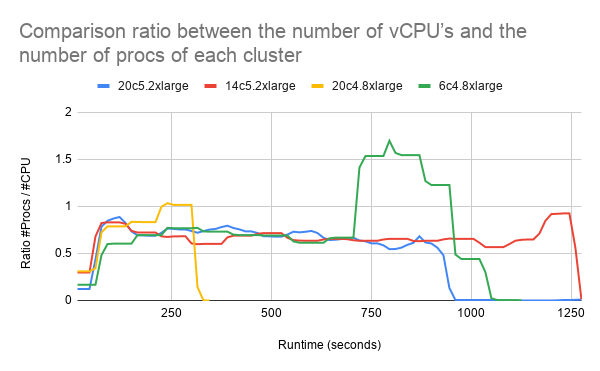
The figure shows that most clusters (besides 6c4.8xlarge) have a similar level of idleness.
With the 6c4.8xlarge cluster we set the number of worker CPU’s to the
number of jobs in the last part of the computation. This number (200
jobs) was found using the Spark History Server. The idea was that the
cluster would for a longer time on a high utilization. In the figure above is visible that a higher utilization was reached in the second part of the computation. Unfortunately, the first
part of the computation had a lower utilization then the other clusters.
In the figure above we can see that 6c4.8xlarge has a
lot more processes than vCPU’s in the second part of the computation.
This might indicate that processes have to wait or share a vCPU which is
not ideal.
Running just with slower instances (c5.2xlarge machines) without any
further tuning leads to a higher utilization, but also increases the run
time significantly. This does not result in lower running costs.
Discussion
During this experiment we encountered that it was quite difficult to analyse the instances individually. Using Ganglia, we were able to export metrics to csv of json format. This however is a manual task. It is not practical to download all the metrics (cpu, memory, network, and load) for all individual instances. We learned that Ganglia stores metric about the instances in RRD files. Unfortunately we were unable to convert (using rrdtool 3) the RRD files to usable csv or json files. Using the RRD files could give us a more fine grained analysis per instance.
Conclusion
When selecting a suitable cluster configuration, the table in the Comparison section can be used to make a decision based on costs and/or idleness. The configuration with 20 c4.8xlarge machines
is the cheapest and fastest option, but the idleness is quite high.
However, when minimizing idleness is the ultimate goal of the company,
it would be a better idea to go with 20 c5.2xlarge machines, but the
cost is slightly higher. The choice might depend on whether the company
owns the cluster itself, and if they do, then it might be a better
option to minimize the idleness. To conclude, there is no ultimate
setup. However, when carefully looking at what happens when the query is
executed, the cluster configuration and the implementation can be tuned
such that the wishes of the company are being fulfilled, without the
result of spending too much money on idle machines.